

Why statistics still matter in crypto anomaly detection
When people hear “crypto anomaly detection”, they often imagine magical AI that spots every scam in real time. In practice, almost every serious crypto anomaly detection software still relies on good old statistics at its core. Machine learning models usually sit on top of statistical features: z‑scores, moving averages, volatility estimates, correlation breakdowns. Without these basic bricks, even the smartest neural network will hallucinate patterns or miss obvious red flags. Understanding these techniques is not just a nerdy hobby: it helps you evaluate vendors, tune alerts, and see when your system is being gamed by sophisticated attackers who know how threshold rules work and actively try to bypass them through splitting payments, wash trading, or timing their actions around low‑liquidity periods.
Key terms, but in plain language
Before diving in, let’s clear up the vocabulary that pops up in every talk about cryptocurrency fraud detection tools. *Anomaly* is anything that statistically deviates from a learned baseline of “normal” behavior. That might be a single strange transaction, but more often it’s a pattern over time: an address suddenly talking to dozens of new counterparties, or an exchange wallet whose withdrawal profile changes overnight. *Baseline* is the statistical model of normality we build from historical data, usually through averages, variances, correlations and seasonal patterns. *False positive* is an alert on something harmless; *false negative* is a real scam that slipped through. Balancing these two is the main daily headache for any risk or compliance team, because tighten thresholds too much and your analysts drown in noise, loosen them and you miss actual fraud that regulators will later point at in audits.
To make sense of time‑dependent behavior, we talk about *time series*: ordered sequences such as hourly on‑chain volumes, rolling balances or gas‑price‑adjusted fees. Crypto blockchains are basically giant time series databases where each block gives a new snapshot of flows. And finally, *entities* vs *addresses*: an on‑chain address is just a key, but an entity is a cluster of addresses controlled by one actor. Most real‑world anomaly detection operates at entity level, because laundering schemes spread behavior over many addresses to dilute the statistical signals you would otherwise easily catch if you only looked at single keys in isolation.
Baseline building: what “normal” looks like in crypto
Any useful blockchain transaction monitoring solutions start with one deceptively simple question: “normal compared to what?”. You cannot call something weird if you never measured the usual pattern. For wallets, normality might mean typical daily transaction count, preferred counterparties, usual assets, and average transaction size with its natural volatility. For centralized exchanges, the baseline includes intraday volume profiles, net inflow and outflow dynamics, and liquidity at various price levels. Because crypto never sleeps, we don’t have weekend vs weekday in the same sense as traditional banks, but we still see strong time‑of‑day cycles and periodic bumps around big news or protocol events.
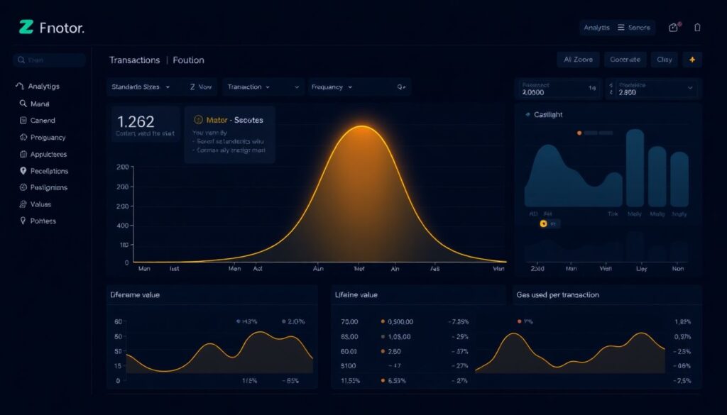
[Diagram: imagine a wavy line showing daily transaction count over 90 days, with a smooth dashed curve running through the middle. The dashed curve is the baseline; the spikes that stick far above are candidate anomalies.]
Statistically, building this baseline often starts with simple moving averages and rolling standard deviations. For example, you can compute a 30‑day moving average of outgoing value for each address and compare today’s outflow against this reference. If today’s value is five or ten standard deviations above the mean, that’s suspicious. More advanced systems add seasonal decomposition: they separate slow trends (growth, accumulation), regular seasonality (daily or weekly patterns), and residual noise. That residual is where anomalies live. This decomposition is especially useful for DeFi protocols, whose usage follows strong cyclical patterns driven by farming incentives, governance votes or predictable liquidations after price shocks.
Core statistical techniques: the toolbox that actually catches stuff
Z‑scores and standard deviation bands
Z‑score is one of the simplest measures but still a workhorse. It tells you how many standard deviations a value is from its mean. In crypto AML compliance analytics platform workflows, z‑scores are applied to transaction sizes, frequency, lifetime value, or even gas used per transaction. If an otherwise quiet address suddenly sends an amount with a z‑score of +8 relative to its past, you can raise an alert without any fancy machine learning. This approach is fast, explainable to regulators, and easy to tune by business stakeholders who are not statisticians, because they intuitively understand “that payment is far outside the normal range we see for that account”.
[Diagram: a bell curve labeled “normal behavior”. In the center is the mean; one, two, and three standard deviation marks are shown on both sides. A red dot far out in the tail is labeled “suspicious transaction with high z‑score”.]
The weakness is obvious: if criminals slowly ramp up their amounts or spread them thin across many wallets, z‑score‑based alerts may never cross your thresholds. This is why experts recommend using z‑scores mostly as a first line of defense or for monitoring relatively stable patterns, like operational hot wallets of an exchange, where any dramatic jump truly is unexpected and harder to disguise behind gradual creeping.
Percentiles and robust statistics
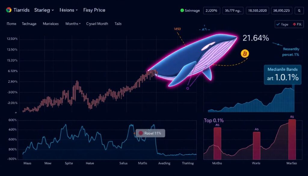
Crypto data is messy and full of fat tails: one giant whale can distort averages for months. Robust statistics deal with this by focusing on medians and percentiles rather than means. Instead of asking “how many standard deviations above average is this value?”, you might ask “is this in the top 0.1% of what we’ve ever seen for this address or cluster?”. This percentile‑based view is common in crypto market manipulation detection system designs, where the distribution of order sizes and cancellation rates is highly skewed.
Using percentiles helps avoid chasing shadows every time a whale moves funds legitimately, because you can filter anomalies based on combined conditions: for example, an order bigger than the 99.9th percentile plus simultaneously happening during a low‑liquidity window and interacting with a small‑cap token. Experts point out that these robust metrics stay more stable over time, which simplifies calibration and reduces the number of times you need to retrain or re‑baseline after a regime change in the market.
Time‑series change‑point detection
Change‑point detection is about spotting moments when the statistical properties of a series abruptly shift: mean jumps, variance spikes, or correlation collapses. In blockchain context, that might look like a wallet whose outgoing transfers suddenly quintuple in both count and size, or a DeFi pool whose inflows and outflows become much more erratic right before an exploit. Algorithms such as CUSUM (cumulative sum), Bayesian change‑point models, or newer non‑parametric methods track cumulative deviations from the baseline until a threshold is crossed.
[Diagram: a time series line that is fairly flat, then at some point jumps to a higher level and stays there. A vertical dashed line marks the detected change‑point.]
Compared to simple threshold rules, change‑point models are better at catching slow burns: activity that escalates over hours or days. This is crucial for detecting “draining” attacks where an adversary is patient, gradually withdrawing liquidity to avoid a single huge spike. Seasoned practitioners advise using at least one change‑point detector in any high‑value monitoring pipeline, especially on exchange hot‑wallet flows and bridge contracts that are frequent targets for sophisticated hackers.
Multivariate models: looking at patterns, not single numbers
Most real‑world fraud schemes only become obvious when you view several dimensions together. A single big withdrawal might be fine; a big withdrawal to a fresh address with ties to a known mixer, during an exchange outage, is less comforting. Multivariate statistical models try to capture the typical joint behavior of features such as transaction count, average size, address age, counterparties, geography, device fingerprints (off‑chain), and token mix.
Classical methods here include Mahalanobis distance, which measures how far a point is from the center of a multivariate distribution while accounting for correlations. In other words, it doesn’t just ask “is the size unusual?” but “is this *combination* of size, timing, and counterparty unusual given everything we know?”. Principal component analysis (PCA) is also popular to reduce dozens of raw metrics to a few orthogonal “factors” like “activity intensity” or “diversity of counterparties”, making anomaly scoring more stable. These techniques sit inside many production cryptocurrency fraud detection tools, usually buried under a marketing layer that talks about “AI‑driven risk scores” but is in fact relying heavily on these explainable mathematical constructs.
Network‑based anomalies: using graph statistics
Blockchains are networks by nature: addresses linked by flows of value. Graph‑theoretic statistics add a powerful angle: instead of only measuring how one address behaves over time, we also look at how it is positioned in the wider transaction graph. Expert teams routinely compute centrality measures (degree, betweenness, PageRank‑style influence), clustering coefficients, and subgraph frequencies. Sudden jumps in these metrics can indicate that an address has become an unexpected hub in a laundering chain or a pivot in a phishing campaign cash‑out path.
[Diagram: a small network of circles (addresses) with lines (transactions). One node in the center suddenly gains many new connections, highlighted in red, indicating an anomalous hub.]
Graph‑based statistics are especially effective against mixers and peel chains—structures where funds move through long sequences of barely used addresses to blur their origin. While any single hop may look harmless in isolation, the overall pattern—a long linear path with nearly identical amounts and short time gaps—is rare in normal retail flows. Statistical pattern‑mining algorithms can flag such structures without needing a priori labels for every mixer smart contract, which is essential in an ecosystem where new obfuscation services appear weekly.
Comparing statistical techniques with pure machine learning
Vendors often promote deep learning as the end‑all solution, but teams that run critical blockchain transaction monitoring solutions tend to mix machine learning with traditional statistics instead of replacing them. Why? First, stats are interpretable: when regulators ask “why did you block this withdrawal?”, you can point to a five‑sigma deviation in average withdrawal size plus a sudden creation of links to sanctioned clusters. A black‑box model that simply outputs “risk score 0.93” is harder to justify, especially in strict jurisdictions.
Second, statistical methods are data‑efficient. Crypto is full of new tokens, new protocols, new behaviors with very little training data. A neural network trained on last year’s DeFi exploits might completely miss an inventive new governance‑attack pattern, while a simple change‑point detector on governance token transfer volumes still has a chance to spot the emerging oddity. Expert practitioners usually view machine learning as an enhancement layer: it learns complex boundaries between “weird but harmless” and “weird and risky” on top of already engineered statistical features, thereby reducing false positives without losing the sharp detection capability of baseline models.
A third practical point: operations. Models must run at scale, often in near real time. A handful of well‑chosen statistical tests can scan millions of events per minute with modest hardware, feeding a shortlist into slower but smarter models. This cascading architecture is a staple in production‑grade crypto anomaly detection software, because it aligns with both budget constraints and latency requirements on high‑throughput chains and busy centralized exchanges.
From math to tools: where these techniques live in practice
When you evaluate crypto monitoring products, the marketing language will talk about “next‑generation AI” and “behavioral analytics”, but under the hood you should actively look for concrete statistical foundations. Mature cryptocurrency fraud detection tools expose or at least document their use of time‑series baselines, volatility bands, percentile‑based risk layers, and graph statistics. They also provide controls to tune sensitivity: sliding thresholds, learn periods, and feature weights. The ability to adjust these is not just a luxury; it is crucial for adapting to regime shifts like bull markets, new regulatory rules, or the sudden rise of a new L2 where fee dynamics differ dramatically from legacy chains.
On the enterprise side, a well‑integrated crypto AML compliance analytics platform typically stitches together on‑chain statistics, off‑chain KYC data, and external risk intelligence such as sanctions lists and darknet tagging. For large financial institutions, the statistical anomaly detection is just one microservice in a longer decision pipeline that also includes case management, analyst feedback loops, and regulatory reporting modules. Each time an analyst clears or confirms a case, that judgment ideally feeds back to refine parameters, telling the statistical engine which patterns are worth prioritizing and which are just noise from legitimate but unusual users.
Expert‑level recommendations for designing your detection stack
To wrap the ideas into something operational, here is a condensed playbook that many experienced monitoring teams informally follow:
1. Start with simple, interpretable metrics.
Begin with z‑scores, percentiles, and rolling averages for each key feature: volume, frequency, counterparties, and graph centrality. Make sure every alert can be explained in one or two sentences referencing these metrics. This builds trust with compliance officers and trains analysts to read the signals correctly before you layer on sophistication.
2. Model behavior at the right granularity.
Experts insist on clustering addresses into entities wherever possible. A single‑address baseline is easy to spoof by rotating keys; entity‑level baselines are much harder to manipulate. Combine this with segmentation: whales, retail users, exchanges, OTC desks, and smart contracts all require distinct baselines because their natural activity patterns differ dramatically.
3. Combine time‑series and graph signals.
Time‑series anomalies (spikes, trend breaks) and network anomalies (weird graph structures) catch different failure modes. Seasoned practitioners rarely rely on just one. Many high‑confidence alerts arise from the intersection: for example, an address that not only shows a sudden withdrawal spike, but also starts participating in a chain‑like pattern common to laundering routes.
4. Layer rules, statistics, and machine learning.
Static rules—like “never allow withdrawals to sanctioned clusters”—are non‑negotiable. Statistical models then catch unknown unknowns, patterns you didn’t foresee when writing rules. On top, supervised ML can learn from labeled alerts which anomalies usually turn out benign and downgrade them, sparing analysts unnecessary workload. This layered approach has proven more robust than any single technique alone.
5. Continuously recalibrate, but cautiously.
Crypto regimes change fast. Experts suggest recalibrating baselines on a rolling window, but with guardrails: keep a long‑term reference so that attackers cannot slowly “boil the frog” by manipulating volumes over weeks. Some teams maintain dual baselines—short‑term and long‑term—and flag deviations where they disagree significantly about what “normal” looks like.
6. Design for false‑positive management from day one.
No matter how clever your statistics, you will generate noisy alerts. Plan triage flows: auto‑close low‑risk anomalies that self‑resolve, group multiple related alerts into single cases, and give analysts rich context (historical charts, entity profiles, and network views) in the same interface. The most successful crypto market manipulation detection system deployments focus as much on workflow ergonomics as on pure detection accuracy.
Future directions: smarter statistics, not blind AI worship
The next few years will likely bring more hybrid models where probabilistic graphs, Bayesian time‑series, and causal inference sit alongside deep learning. Instead of just pattern matching past scams, systems will try to reason about what *caused* a pattern: was it a protocol upgrade, a coordinated pump‑and‑dump campaign, or simply organic adoption? Better causal statistics can reduce overreaction to harmless spikes and sharpen focus on intentional manipulation.
At the same time, transparency pressure will only increase. Regulators already ask probing questions about how decisions are made in automated monitoring systems, and users push back against opaque account freezes. This climate favors approaches where the statistical reasoning can be surfaced clearly: charts of baselines, evidence of shift points, graphs of anomalous clusters. Teams that invest now in explainable, statistically grounded crypto anomaly detection software will be better positioned than those who chase the latest black‑box trend without understanding the math beneath.